- The Sovereign Climate Risk Rating (SovCRR) translates chronic physical climate risk into expected GDP-percapita impacts.
- Damages are estimated at the sub-national level before being aggregated nationally.
- Regional damage estimates are aligned with NGFS scenarios and probability-weighted outputs.
- A US case study is presented, showing greater GDP risks for southern states than for northern peers by 2050
Sovereign climate-risk measures typically begin with country averages and end in composite scores. The Sovereign Climate Risk Rating (SovCRR) follows the opposite route. It begins with historical temperature and output records observed at the subnational level, projects the resulting damages across more than 3,400 regions, translates those estimates into nine probabilistic pathways aligned with the Network for Greening the Financial System (NGFS) and only then aggregates them into a probability-weighted countrylevel expected loss or gain that feeds into an A–G rating. This article explains this stepwise construction. It outlines the underlying scientific methodology, illustrates its application to the US and highlights SovCRR’s distinctive features. The letter grade is an important reporting layer; beneath it lies a transparent, scenario-consistent and probabilityweighted estimate of the future impact of chronic physical climate risk on GDP per capita.
Sovereign climate risk faces an aggregation problem
Climate change is a public good problem, but it is also a distribution problem. Why? Our changing climate is affecting all regions globally, leaving no economic region or unit untreated, but its expected economic materiality will be heterogeneous across space. National economies are clusters of regions spanning different climate zones, sectoral structures, population patterns and sensitivities to additional warming. Collapsing these differences into a national average before estimating damages can therefore produce a misleading result because it does not accurately reflect the heterogeneous distribution of economic activity within countries. The problem is especially relevant because the temperature-output relationship has been found to be non-linear by the scientific literature (Burke et al [2015]): a one-degree increase does not have the same marginal effect in a cool region as in an already-hot one, and moderate gains in cooler areas may not offset the substantial losses predicted in warmer ones.
This matters for sovereign portfolios because climate risk enters credit analysis through economic fundamentals. Persistent productivity losses can weaken the potential output path and, over time, the tax base and fiscal capacity on which debt service ultimately depends. Yet the climate information available to investors is commonly either (i) too aggregated for heterogeneous countries or (ii) expressed as a vulnerability index whose economic meaning is difficult to connect to an existing country-risk model. Moreover, because chronic physical climate risks1 remain insufficiently reflected in market prices, investors need forward-looking, non-market data to identify structural economic vulnerabilities before they materialise in sovereign credit spreads.
SovCRR addresses these limitations through a focused, economically interpretable and geographically granular measure: the projected change (reduction or increase) in GDP per capita attributable to climate change-driven shifts in average temperature (ie, the central component of chronic physical risk), relative to a counterfactual without further climate change, at the 2035 and 2050 horizons. This direct link between climate exposure and macroeconomic outcomes distinguishes SovCRR from broader vulnerability indices and makes its results readily ingestible into the models of sovereign credit analysts. The current version of SovCRR deliberately isolates this temperature-economy channel.
In recent decades, the scientific literature estimating the true macroeconomic cost of climate change has treated it primarily as a public good problem. A stable climate is non-excludable and largely non-rival. While greenhouse gas emissions generate global externalities, exposure to and damages from climatedriven shifts in average temperature vary substantially across space. This leaves no productive units and geographic locations untreated per se. As a result, statisticians have typically relied on the local variability of historical climate fields over time to econometrically predict country- or region-level GDP deviations (Burke et al [2015]; Kalkuhl and Wenz [2020]; Linsenmeier [2023]; Berg et al [2024]; Kotz et al [2024], among others). This approach, backed by a long line of increasingly granular studies, has structured the applied physical-risk modules used by institutions, central banks and scenario providers in financialrisk and stress-testing frameworks. For example, Oxford Economics (2022) uses Burke et al (2015); earlier NGFS vintages used Kalkuhl and Wenz (2020); and the latest Phase V used Kotz et al (2024). This ‘local’ approach2 has provided a natural foundation for the EDHEC Climate Institute’s applied scientific developments, notably the methodology developed in Schneider (2026a), which underpins the first two stages presented below.
Outline of the methodology: how the SovCRR is built
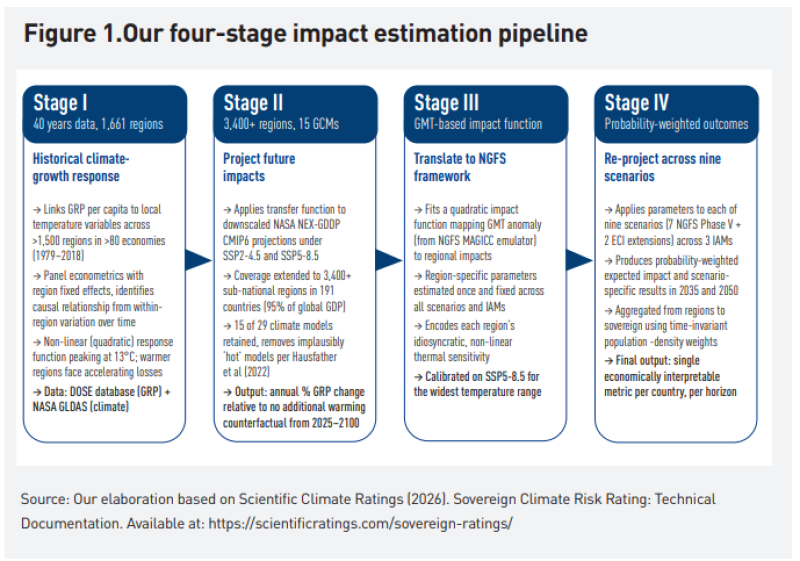
The model is organised as a four-stage pipeline that moves from historical identification to future regional damages, then from climate scenarios to a sovereign-level decision metric. Each stage has a distinct role, which makes the assumptions, degrees of freedom and potential sources of uncertainty easier to identify.
Stage 1: estimate how regional growth has responded to climate
The first stage combines roughly four decades of harmonised gross regional product (GRP) per capita data from the MCC-PIK Database of Subnational Economic Output with local temperature and precipitation records from NASA’s Global Land Data Assimilation System (Wenz et al [2023]). Gridded climate observations are matched to administrative regions using geographic boundaries and population-density weights. The estimation panel covers more than 1,500 regions in 87 countries and identifies the relationship using variation within regions over time, with region-specific time trends absorbing persistent cross-sectional differences.
The resulting transfer function is non-linear and concave, consistent with the established climate-economy literature. The benchmark response peaks at an annual average temperature threshold: regions below that level may initially experience small gains or limited losses, while regions already above it face increasingly negative marginal effects as temperatures rise. Lagged responses allow temporary growth shocks to cumulate into lasting differences in the level of output per person.
Stage 2: project the response across future local climates
The estimated historical relationship is applied to NASA’s bias-corrected and downscaled NEX-GDDP-CMIP6 projections (Thrasher et al [2022]). This extends the calculation to more than 3,400 sub-national regions in 191 sovereign economies, representing more than 95% of global economic output. The original climate ensemble contains 29 global climate models. For the production estimate, 14 models are retained after screening out models whose equilibrium climate sensitivity or transient climate response lies outside the ranges assessed as likely in the climate literature (Hausfather et al [2022]).
For each region, future temperature changes are measured against the 1980–2010 climate baseline and fed into the transfer function. Physical riskinduced transient productivity growth shocks are cumulatively compounded over time, yielding a permanent gap in the level of GRP per capita relative to a no-additional-warming counterfactual. The underlying research engine spans 2025–2100, although the current rating focuses on 2035 and 2050 because these horizons are more financially relevant.
Stage 3: translate SSP-RCP damages into the NGFS architecture
The economic changes predicted in Stage 2 are, by nature, expressed under SSP-RCP pathways and individual global climate models. Banks and institutions, by contrast, commonly rely on the NGFS framework. SovCRR therefore introduces a translation layer rather than assigning each NGFS scenario mechanically to a single SSP-RCP path. For every region, a non-linear aggregate damage function relates projected damage to GRP per capita to the change in global mean temperature emulated by the MAGICC module. In line with NGFS (2024), the initial calibration uses high-emission pathways to span the widest available temperature range, and the function is estimated without an intercept because damages are defined relative to the climate-neutral (no additional climate impact) counterfactual.
This produces more than 3,400 unique region-specific parameter pairs. They are estimated once, but can be applied across NGFS scenarios, the three integrated assessment models (IAMs) used by NGFS, and projection years. The parameters, which are spatially varying but stable across scenarios, preserve the locationspecific non-linearity, persistence and climate-model information embedded in Stage 2 damage trajectories, while making those trajectories compatible with different scenario architectures.
Stage 4: re-project, aggregate and calculate the unconditional expected loss using scenario probabilities
The regional parameters are applied to annual MAGICC temperature paths across nine forward-looking scenarios: the seven NGFS Phase V scenarios and two higher-warming extensions, Climate Destabilisation and Climate Breakdown from Scientific Climate Scenarios.3 The result is a complete scenario-by-IAM matrix of annual regional damage paths. Those paths are aggregated from regions to countries using time-invariant population-density weights from the Gridded Population of the World dataset, so that the spatial distribution of economic agents, which tends to coincide with that of productive activity, matters to the sovereign total.
For each scenario, impacts are averaged across the three IAMs. Unequal scenario probabilities are then applied to calculate an unconditional expected impact for each country and horizon (Rebonato et al [2025]). This expected-impact estimate complements rather than replaces stress testing: all nine scenario-specific estimates remain available. But by moving beyond the conventional ‘what if?’ logic of scenario analysis to assess ‘what is likely or expected?’, SovCRR provides a decisionuseful measure of the financial materiality of chronic physical risk for sovereign markets. Investors can therefore directly integrate a probability-weighted estimate of climate-related economic damage into their sovereign-risk models. A chart summarising this stepwise methodology (ie, identify, project, translate, aggregate) is given in figure 1.
From a predicted economic impact to an A-G risk rating
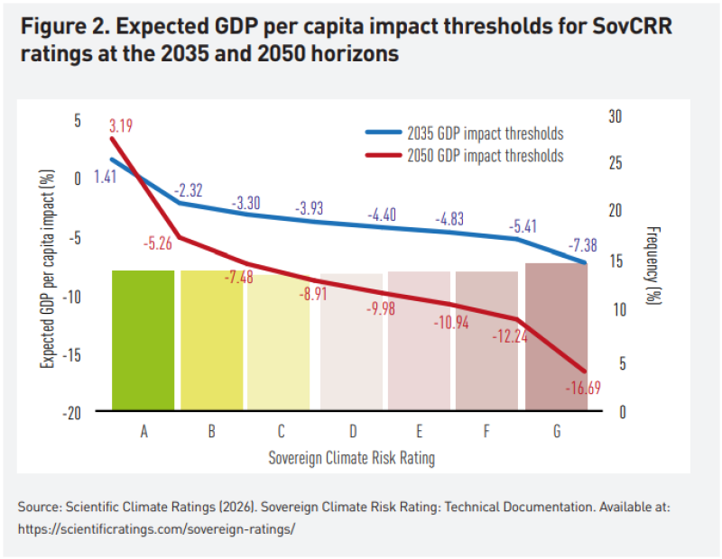
The most important design choice is that the rating does not replace the economic metric. For every country, SovCRR first reports the expected cumulative impact on GDP per capita, in percentage terms, at the 2035 and 2050 horizons. Countries are ranked by that impact and placed into seven approximately equal rating bands from A to G, based on percentile scores ranging from 1 to 100. A denotes the least exposed part of the rated universe and G the most exposed. Horizon-specific thresholds for 2035 and 2050 are calibrated on the expected-scenario distribution and applied consistently to scenario-specific results at the same horizon. These thresholds are naturally versioned and will be recalculated whenever the universe or data change.
Each rating is anchored to horizonspecific thresholds for the probabilityweighted expected loss across nine scenarios. The E band lies between approximately –4.4% and –4.8% in 2035 and between –10.0% and –10.9% in 2050, reflecting the compounding of climate impacts over time. A graph representing the expected GDP per capita impact thresholds for SovCRR ratings at the 2035 and 2050 horizons is given in figure 2.
This architecture separates measurement from communication. The percentage impact is the economically interpretable quantity that can enter a macroeconomic forecast, a sovereign-credit overlay or a stress-testing model. The 1–100 score and A–G grade make cross-country screening and governance easier. Users retain access to the underlying scenario results, annual paths and sub-national decomposition, so two countries with the same letter grade need not be treated as economically identical. Comparisons can also be organised by climate zone, market group or geographical region rather than relying only on a global rank.
Why the approach is distinctive for sovereign investors
Sovereign pricing tends to respond more strongly to acute climate shocks and transition signals than to gradual, temperature-driven productivity losses. Existing frameworks often provide vulnerability rankings or stress-test results rather than expected economic impacts, while national averages can mask the concentration of activity in exposed regions. SovCRR addresses these limitations in four ways.
First, it expresses chronic physical risk as an explicit percentage impact on GDP per capita. This metric can be incorporated into macroeconomic forecasts, debt-sustainability analysis and sovereign scorecards, with investors applying their own assumptions to translate output effects into fiscal balances, debt dynamics and spreads.
Second, SovCRR estimates damages at the sub-national level before aggregating them nationally. This captures the spatial distribution of climate exposure and economic activity and reveals whether a sovereign’s risk is broad-based or concentrated in particular regions.
Third, SovCRR re-projects its own region-specific damage functions across the seven NGFS Phase V scenarios and two higher-warming extensions, rather than using the NGFS physical-damage estimates (NGFS [2024]; Schneider [2026b]). It therefore provides both scenario-specific results for stress testing and a probability-weighted expected impact for portfolio analysis.
Finally, the methodology remains traceable. The letter grade can be linked back to GDP per capita impacts, scenario paths and sub-national drivers, supporting model validation and informed adjustments (Scientific Climate Ratings [2026]).
A practical illustration: the US
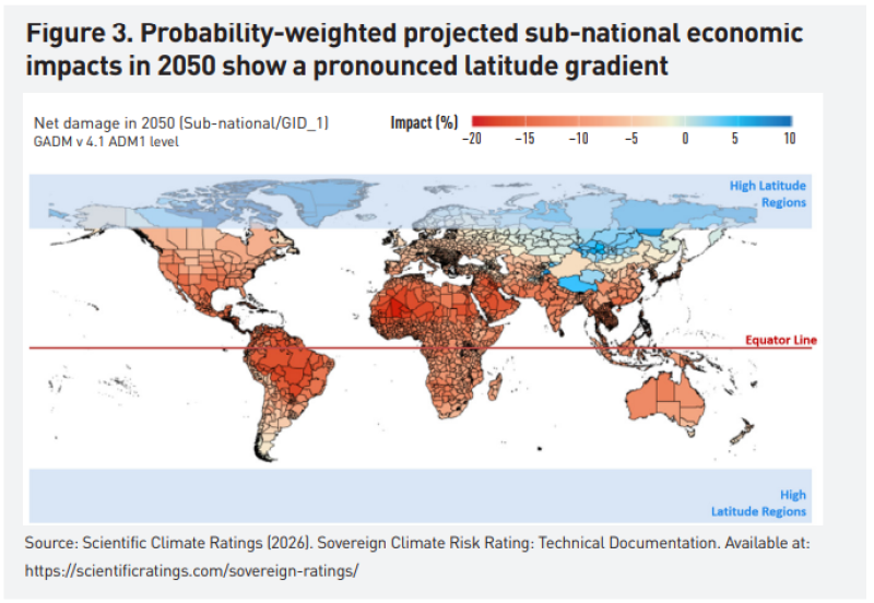
The US illustrates the importance of modelling climate damages below the national level. A map showing the spatial distribution of probability-weighted projected sub-national economic impacts in 2050 (globally) is presented in figure 3. Its average temperature lies just below the globally estimated optimum and could therefore make a national damage function appear relatively benign. Yet more than 40% of US economic activity is concentrated in southern states that already exceed the literature threshold, beyond which the response curve becomes markedly steeper. Cooler northern states may initially benefit from warming, but these gains remain smaller than the accelerating losses in warmer states. This domestic asymmetry reflects the broader latitude gradient observed globally, with larger losses generally concentrated in warmer, lower-latitude regions.
The state-level estimates make this contrast explicit. Figure 4 shows the US national rating and selected state-level impacts based on the unconditional expectation. Under this probabilityweighted expectation, GRP per capita losses by 2050 reach approximately 13.7% in both Arizona and Texas, compared with 7.5% in New York and 7.7% in Minnesota. California and Florida record losses of 11.0% and 10.1%, respectively. Because economic activity is unevenly distributed and the temperature-productivity relationship is concave, northern and southern states do not provide a natural hedge when aggregated.
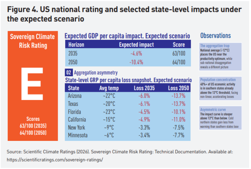
At the national level, the methodology estimates a US GDP per capita impact of –4.6% by 2035 and –10.4% by 2050, corresponding to scores of 63/100 and 64/100 and an E rating at both horizons. The scenario range remains relatively narrow in 2035 but widens substantially by 2050, when the US impact ranges from approximately –4.1% under Low Demand to –14.9% under Climate Breakdown. For investors, the central estimate therefore captures a material structural impact rather than a stress scenario, while the wider distribution shows the additional tail risk. A national average alone would obscure the regional composition underlying both.
Scope, limitations and next developments for the product
A product is more credible when its boundaries are explicit. SovCRR Version 1 measures exposure to chronic, temperature-driven productivity risk. Acute hazards are not modelled separately, although part of their historical economic signal may be embedded in the estimates. Top-down panel models identify the aggregate relationship between observed temperature variation and GDP, making it difficult to disentangle the effects of gradual warming from those of correlated acute extremes. The estimates may therefore capture elements of both, even though the model does not represent individual hazards explicitly. Tipping points are excluded. Dell et al (2014) provide a broader review of this empirical literature.
These limitations also define a research and product agenda. First, sector-specific macroeconomic damage functions would reveal which segments in the overall composition of economic activity drive sovereign exposure. A second priority is to separate direct losses from their propagation through supply chains. The financial materiality of physical climate risk extends beyond firms’ direct climatic exposure because correlated disruptions can spread through production networks and inter-firm spillovers. Empirical damage estimates based on local temperature variability may capture some of these indirect effects through observed GDP, but the associated ‘damage delta’ cannot yet be reliably isolated or formally quantified. A third priority is to model future adaptation explicitly; current projections hold adaptation margins fixed at their historically observed levels. Most importantly, calibrating the translation from output losses to sovereign credit ratings and spreads would move the framework closer to valuation.
The existing design and the EDHEC Climate Institute research agenda are intended to allow these extensions to be introduced incrementally.
Conclusion
SovCRR’s principal innovation is a continuous analytical chain from historical climate and economic records to forward-looking, probability-weighted sovereign risk metrics. By estimating damages at the sub-national level before aggregation, translating them consistently across NGFS-aligned scenarios and keeping GDP per capita impacts visible beneath the rating, the framework preserves the economic information needed for credit analysis rather than reducing climate exposure to a standalone score.
For investors, this creates a practical bridge between physical climate risk research and sovereign portfolio decisions. The expected losses can enter macroeconomic forecasts, fiscal analysis and debt-sustainability assessments, while the scenario distribution and regional decomposition reveal the sources and tails of risk. The rating simplifies comparison, but the underlying metric remains traceable. This combination of granularity, scenario consistency and economic interpretability makes SovCRR a distinctive tool for the early identification of the structural vulnerabilities of economies before they are priced into sovereign credit spreads.
SovCRR is designed for several user groups. Institutional investors can use it to quantify climate-related sovereign risk in terms compatible with portfolio and credit models; banks and developmentfinance institutions can demonstrate climate-risk integration using interpretable economic metrics rather than standalone scores; public-sector and supranational institutions can compare climate-vulnerable countries on a consistent, financially grounded basis; and corporate treasuries can assess the climate dimension of their sovereign holdings and geographically concentrated revenues.
References
- Berg, K. A., C. C. Curtis and N. C. Mark (2024). GDP and temperature: Evidence on cross-country response heterogeneity. European Economic Review 169.
- Bilal, A., and D. R. Känzig (2026). The macroeconomic impact of climate change: Global versus local temperature. The Quarterly Journal of Economics 141(2): 889-994.
- Burke, M., S. M. Hsiang and E. Miguel (2015). Global non-linear effect of temperature on economic production. Nature 527: 235-239.
- Dell, M., B. F. Jones and B. A. Olken (2014). What do we learn from the weather? The new climate-economy literature. Journal of Economic Literature 52(3): 740-798.
- Hausfather, Z., K. Marvel, G. A. Schmidt, J. W. Nielsen
- Gammon and M. Zelinka (2022). Climate simulations: Recognize the ‘hot model’ problem. Nature 605: 26-29.
- Kalkuhl, M., and L. Wenz (2020). The impact of climate conditions on economic production: Evidence from a global panel of regions. Journal of Environmental Economics and Management 103: 102360.
- Kotz, M., A. Levermann and L. Wenz (2024). Retracted article: The economic commitment of climate change. Nature 628(8008): 551-557.
- Linsenmeier, M. (2023). Temperature variability and long-run economic development. Journal of Environmental Economics and Management 121: 102840.
- Network for Greening the Financial System (2024). NGFS Climate Scenarios for central banks and supervisors: Phase V – Technical documentation.
- Oxford Economics (2022): https://www.oxfordeconomics. com/resource/the-global-economic-costs-of-climateinaction/ and https://www.oxfordeconomics.com/resource/ estimating-the-economic-impact-of-temperaturevolatility/
- Rebonato, R., L. Melin and F. Zhang (2025). Climate scenarios with probabilities via maximum entropy and indirect elicitation. SSRN Working Paper 5128228.
- Schneider, N. (2026a). The global geography of long-term projected macroeconomic damages from chronic physical risk and the aggregation problem. Cambridge Elements in Quantitative Finance forthcoming.
- Schneider, N. (2026b). A method for reprojecting SSP-RCP damages under NGFS scenarios x IAM trajectories. EDHEC Climate Institute Technical Note.
- Schneider, N. (2026c). The global versus local identification of macroeconomic damages: Signal, assumptions, uncertainty. EDHEC Climate Institute Position Paper. Scientific Climate Ratings (2026).
- Sovereign Climate Risk Rating: Technical Documentation. Available at https:// scientificratings.com/sovereign-ratings/
- Thrasher, B., W. Wang, A. Michaelis, F. Melton, T. Lee and R. Nemani (2022). NASA Global Daily Downscaled Projections, CMIP6. Scientific Data 9: 262.
- Wenz, L., R. D. Carr, N. Kögel, M. Kotz and M Kalkuhl (2023). DOSE – Global data set of reported sub-national economic output. Scientific Data 10: 425