EDHEC-CLIRMAP unveils wide disparity in state damages depending on climate zones

In this article, we review the variances of geographic and climate extremes present in the US (Section 1) and use the EDHEC-CLIRMAP tool to explore the economic implications of climate change across the US (Section 2). 

We interpret the regional patterns produced by this model, discuss plausible underlying acute drivers that are not directly observed in the framework, and list the types of financial materiality that may emerge from these projected macroeconomic impacts.

The sign and magnitude of predicted economic losses are determined by the intersection between space, through local climate zones and baseline temperature conditions, and the non-linear temperature–GDP structural relationship estimated in the underlying EDHEC-CLIRMAP methodology. The location of a given region therefore matters because it determines where that region sits on the response curve, and whether additional warming is projected to generate limited effects, temporary gains, or increasingly negative economic impacts.

Accordingly, different states are likely to see massive variations in the resulting economic impact. Southern states are particularly vulnerable to more intense and frequent extreme heat waves, with heightened risks of water shortages and wildfires occurrence. By contrast, high-latitude temperate states, such as those in the northern continental US, will experience more moderated cold-season low-temperature extremes. In some zonal areas, climate change will extend the length of growing seasons, offering potential benefits for agriculture. In others, proportionally larger temperature increases will push local climate conditions away from the historical baseline, challenging local ecosystems. For example, Florida’s exposure to the likes of storms, wildfires, extreme heat and rising sea levels could wipe more than a quarter off its GRP by the end of the century, and the forecasts are similar for California. The numbers for Texas are even more concerning; gross regional economic product (GRP) damages could reach 43% by 2099 as storms, flooding, droughts and heat take their toll. 

EDHEC-CLIRMAP (EDHEC-CLimate-Induced Regional MAcroimpacts Projector) is a free online tool developed by the EDHEC Climate Institute. Scientists, experts, professional investors, policymakers, and ordinary users can use this free user-friendly platform to discover how climate change–induced shifts in average temperature are projected to affect the GRP of individual regions.

Background

Climate change is happening all around us, sparing no region or industry. Its impact will be determined by the urgency with which nations take action to rein in and slow anthropogenic emission drivers and ultimately adapt to gradually reduce its cost to society. 

These risks (and their underlying materiality) are expected to vary significantly across regions (and implicitly, climate zones). The US provides an ideal illustration of this observation, with its wide geography and strong climate extremes – from hot to cold deserts, forests, mountains, flat and cliff-edge coasts, the near equatorial regions of southern states, and the permafrost of Alaska. 

In this article, we review the heterogeneity of geographic and climate extremes present in the US. We summarise the acute and chronic risks that climate change is bringing to bear and their impact, such as fiercer storms, more frequent and intense wildfires, and rising sea levels. We outline the mechanisms through which these impacts may financially materialize. 

In this article, we use the EDHEC-CLIRMAP tool to project GRP shocks in a selection of the states that are likely to be the hardest hit by this risk evolution.

We interpret the regional patterns produced by the model, discuss plausible underlying acute drivers that are not directly observed in the framework, and list the types of financial materiality that may emerge from these projected macroeconomic impacts.

The sign and magnitude of predicted economic losses are determined by the intersection between space, through local climate zones and baseline temperature conditions, and the non-linear temperature–GDP structural relationship estimated in the underlying EDHEC-CLIRMAP methodology. The location of a given region therefore matters because it determines where that region sits on the response curve, and whether additional warming is projected to generate limited effects, temporary gains, or increasingly negative economic impacts.

Climate change is a financially material risk exerting economically meaningful pressure on firm performance. Climate change is shifting the distribution of extreme heat events, making them more intense and frequent over time. While acute physical risks compile discrete extreme events such as hurricanes and floods and capture immediate headlines, chronic physical risks (long-term shifts in temperature patterns, precipitation regimes and sea-level rise) pose equally significant challenges through gradual effects to sectoral productivity, asset values, and financial stability. 

Importantly, the macroeconomic damage function literature typically refers to chronic risks (particularly changes in average temperature, whether local or global), but it may also be considered as capturing acute risk impact on GDP, since these are computed from a top-down perspective, and chronic-vs-acute effects cannot be clearly disentangled. Hence, estimates derived from the CLIRMAP methodology, and presented in this article, capture the long-run macroeconomic impacts from both the chronic gradual increase in temperatures and the correlated increase in acute extreme climatic events combined. Tipping points are however excluded.

Review of the US Climate Zones 

Geographical extremes in the US 

North and South:

• Alaska: Northern most state, just 2,000km south of the North Pole.
• Hawaii: Southern most state, just 2,100km north of the Equator.

High and low:

• Mount Denali, Alaska: highest peak at 6,190m.
• Death Valley, California: lowest point at -86m.

Hot and cold

• Great Basin desert: coldest desert in the US due to elevation (mostly above 1,200m with peak at 3,000m) drops low as -7.3°C in winter.
• Chihuahuan desert: largest desert in North America at ~360,000km² (though mostly in Mexico)
• Sonoran: lushest desert, with more plant species than any desert in the world.
• Mojave: hottest desert, home to Death Valley, the hottest place ever recorded (56.7°C in 1913).
• Utqiaġvik, Alaska: the coldest inhabited place in the US, with winter temperatures that average -24°C. All-time record low of -62°C was recorded at Prospect Creek Camp in 1971.

Wet and dry

• Hawaii: wettest state with a mean average of 161.8cm of rain a year. Its volcanic mountains wring moisture out of trade winds.
• Nevada: driest state by far with just 24.1 cm a year. Mountain ranges block Pacific moisture from the desert or high-altitude region of the interior West. 

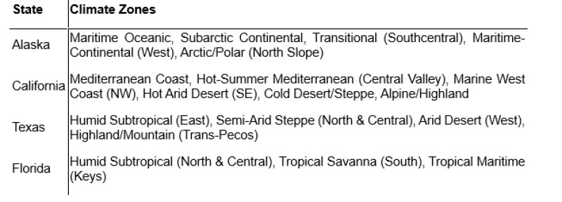
The climate of the US varies hugely, not just from North to South, but within individual states, many of which contain multiple climate zones. The standard classification system for Climate Zones is the Köppen-Geiger framework, which breaks zones into five major groups, each subdivided by temperature and rainfall seasonality:

A:               Tropical: All months above 18°C. High annual rainfall (1.5+ metres). No true winter. Found in South Florida, Hawaii, and US territories. Subdivides into rainforest (Af), monsoon (Am), and savanna (Aw).

B:               Dry (Arid & Semi-Arid): Evaporation consistently exceeds precipitation. Hot deserts (BWh) in the SW; cold deserts (BWk) at elevation. Semi-arid steppes (BS) cover the Great Plains and Great Basin. Covers roughly a third of the contiguous US.

C:               Temperate: Coldest month between -3°C and 18°C. Includes humid subtropical (Cfa) across the Southeast, Mediterranean (Csa/Csb) along the California coast, and oceanic (Cfb) in the Pacific Northwest.

D:               Continental: At least one month below -3°C; no dry season (f) or dry summer (s). Warm summers (a), cool summers (b), or subarctic (c/d). Dominates the Midwest, Great Lakes, and much of Alaska’s interior.

E:               Polar: No month reaches 10°C. Tundra (ET) has at least one month above freezing; ice cap (EF) does not. Found across Arctic Alaska and at high alpine summits.

H:               Highland: This is a useful supplementary classification for mountainous terrain (such as the Rockies, Sierra Nevada, Cascades and Alaska Range) where rapid changes in elevation create highly localised climates that don’t neatly fit into the core groups.

Table 1: Some states with multiple climate zones

Physical climate risks 

While the risks brought by climate change are numerous and interconnected, NOAA (National Oceanic and Atmospheric Administration) considers the following to be the 10 most major, based on its monitoring of “billion-dollar disasters” and climate impacts:

1. Increased Frequency of Severe Storms 
2. More Intense and Wetter Hurricanes 
3. Destructive Coastal Flooding and Storm Surge
4. Prolonged and Intense Drought
5. Intensified Wildfire Seasons
6. Extreme Heatwaves
7. Inland Flooding from Heavy Rainfall
8. Ocean Acidification
9. Shrinking Sea Ice and Glaciers
10. Significant Ecosystem and Biodiversity Disruption

Within this array, it’s also useful to understand the difference between acute and chronic climate risks. 

• Acute risks are event-driven, such as sudden, discrete weather events of short duration but high intensity. Examples include hurricanes, floods, wildfires, heatwaves, and extreme precipitation. They tend to cause concentrated, visible damage in a short timeframe.
• Chronic climate risks are gradual, longer-term shifts in climate patterns that progressively alter conditions over years or decades. Examples include rising sea levels, increasing average temperatures, changing rainfall patterns, and permafrost melt. The damage is cumulative rather than sudden.

It’s also worth noting that the two interact; the frequency and severity of each type of risk may vary considerably and become increasingly difficult to predict, and the drivers may appear with a significant time lag.

US States Through the EDHEC-CLIRMAP Lens

Throughout the rest of this article, we use the EDHEC-CLIRMAP tool to look at specific US-State cases. Note that we interpret the regional patterns produced by the model, discuss plausible underlying drivers that are not directly observed in the framework, and list the types of financial materiality that may emerge from these projected macroeconomic impacts. 

The reason is that the macroeconomic damage function literature typically refers to chronic risks (particularly changes in average temperature, whether local or global), but it may also be considered as capturing acute risk impact on GDP, since these are computed from a top-down perspective, and chronic-vs-acute effects cannot be clearly disentangled. Hence, estimates derived from the CLIRMAP methodology, and presented in this article, capture the long-run macroeconomic impacts from both the chronic gradual increase in temperatures and the correlated increase in acute extreme climatic events combined. Tipping points are however excluded. Recall that the sign and magnitude of predicted economic losses are determined by the intersection between space, through local climate zones and baseline temperature conditions, and the non-linear temperature–GDP structural relationship estimated in the underlying EDHEC-CLIRMAP methodology. The location of a given region therefore matters because it determines where that region sits on the response curve, and whether additional warming is projected to generate limited effects, temporary gains, or increasingly negative economic impacts.

What is the underlying methodology to these losses?

EDHEC-CLIRMAP was built in two stages:

Stage 1: estimate how regional growth has responded to climate

The first stage combines roughly four decades of harmonized gross regional product (GRP) per capita data from the MCC-PIK Database of Subnational Economic Output with local temperature and precipitation records from NASA’s Global Land Data Assimilation System. Gridded climate observations are matched to administrative regions using geographic boundaries and population-density weights. The estimation panel covers more than 1,500 regions in 87 countries and identifies the relationship using variation within regions over time, with region-specific time trends absorbing persistent cross-sectional differences.

The resulting transfer function is non-linear and concave, consistent with the established climate-economy literature. The benchmark response peaks at an annual average temperature threshold: regions below that level may initially experience small gains or limited losses, while regions already above it face increasingly negative marginal effects as temperatures rise. Lagged responses allow temporary growth shocks to cumulate into lasting differences in the level of output per person.

Stage 2: project the response across future local climates

The estimated historical relationship is applied to NASA’s bias-corrected and downscaled NEX-GDDP-CMIP6 projections. This extends the calculation to more than 3,400 sub-national regions in 191 sovereign economies, representing more than 95% of global economic output. The original climate ensemble contains 29 global climate models. For the production estimate, 14 models are retained after screening out models whose equilibrium climate sensitivity or transient climate response lies outside the ranges assessed as likely in the climate literature (Hausfather et al., 2022).

For each region, future temperature changes are measured against the 1980-2010 climate baseline and fed into the transfer function. Physical-risk-induced transient productivity growth shocks are cumulatively compounded over time, yielding a permanent gap in the level of GRP per capita relative to a no-additional-warming counterfactual. The underlying research engine spans 2025-2100. 

Storms

Storms vary in type and intensity:

Thunderstorms range in severity from single-cell storms to supercells, which can be up to 24km wide with winds over 130km/h. Heavy rain can cause flooding, while lightning can trigger wildfires. Lightning strikes the US about 25 million times a year.

Tornadoes are narrow, violently rotating columns of air spawned by supercell thunderstorms. Wind speeds may reach 160 to 480 km/h and cause havoc on the ground. Most spawn in the Central Plains during spring and early summer, when warm, moist air from the Gulf of Mexico clashes with cold, dry continental air from the northwest. 

Hurricanes (also known as tropical cyclones or typhoons) form over tropical or subtropical waters and gain their energy from warm ocean waters. They are about a thousand times larger than tornadoes – 100km to over 1,600km across – and may travel thousands of kilometres over days or weeks. 

Derechos (“inland hurricanes”) are wind storms associated with a band of rapidly moving thunderstorms. The winds can be as strong as those found in hurricanes or even tornadoes but follow straight lines. They are most common in the Midwest and Great Plains in summer and can travel hundreds of kilometres in hours.

Hailstorms. While these are not a separate storm type, but a hazard produced by severe thunderstorms, it is worth mentioning them separately as they cause specific damages, particularly to crops where their effect can be devastating.

Regional exposures vary massively, but some states are particularly affected:

• Texas: highest number of tornadoes annually, averaging over 155 per year.
• Oklahoma: tops the charts for the strongest tornadoes, with catastrophic damage recorded around Moore and Oklahoma City. 
• Florida, no contest hurricane capital: 125 of the 308 hurricanes that buffeted the US from 1851 to 2022 hit Florida.
• Florida again, thunderstorms & lightning: Florida has the highest number of “thunder days” of any state, at 80-105+ a year.

Storm damage

Hurricanes are the costliest storm type. Between January 1980 and July 2020, they accounted for more than half of all billion-dollar disaster damages in the US, which totalled $1.79 trillion across 273 events. The mechanisms are multiple and compound each other: wind destroys structures; storm surge inundates coastlines; extreme rainfall causes inland flooding; and spawned tornadoes extend damage hundreds of kilometres from the storm’s central path. Hurricanes also trigger supply chain disruption, ecological changes, pollution and crop damage. Tornadoes cause intense but geographically concentrated damage, primarily structural destruction from extreme wind. Major storms in general – including hail, high winds, and lightning – are the most frequent billion-dollar event type.

How climate change is shifting storm occurrence

The key finding is that total storm frequency may not increase dramatically, but more intense storms are forming. Warmer oceans act as fuel for hurricanes, so the proportion reaching the most powerful categories (4 and 5) is rising. 

• Maximum wind speeds generated by roughly 80% of Atlantic Basin hurricanes from 2019 to 2023 have intensified by an average of 29kph. Potential damages from winds increase by roughly four times with each jump in hurricane category, so even a modest intensity increase translates to dramatically higher damage.
• Warmer sea temperatures produce wetter hurricanes, with 10–15% more precipitation projected from storms. Recent examples include Hurricane Harvey (2017, over 152cm in some locations), Florence (2018, over 89cm), and Imelda (2019, 112 cm).
• Geographic shift: Storms are peaking further north, potentially putting previously less-exposed states at greater risk. Tornadoes are also migrating, with fewer occurring in the traditional “Tornado Alley” states but more hitting Mississippi, Alabama, Arkansas, Missouri, Illinois, Indiana, Tennessee, and Kentucky. This eastward shift matters enormously for risk, because the Southeast is more densely populated. The tornado season is also getting longer.

GRP damage mechanisms of storms

NOAA estimates an average cost of $22.8 billion per hurricane. The 2024 hurricane season produced an estimated $500 billion in total damage and economic loss, one of the costliest on record. The mechanisms through which storms hit GDP and GRP are layered:

Acute risks: 

• Direct asset destruction interrupts production immediately.
• Labour market disruption shrinks employment through displacement and business shutdowns. A single Category 5 hurricane could decrease annualised quarterly GDP growth by 0.14%.
• Supply chain disruption radiates damage nationally. Indirect effects, such as long-term disruptions to trade, employment, and productivity, are often more destructive than direct damages.
• Sectoral impacts hit tourism, hospitality, agriculture, and construction hardest.

Chronic risks:

• Warmer oceans fuel rapid intensification, the key cost driver. Some 70% of US billion-dollar tropical cyclones since 1980 underwent rapid intensification, and the five most costly, with combined damages of around $680 billion, all intensified at extreme rates. Cyclone intensification losses are estimated at 0.07% of annual GDP per 1°C of warming, compounding with every degree.
• Severe storm costs are escalating structurally. The average annual cost of billion-dollar severe storms rose from $3.8 billion (1985–2004) to $21.8 billion (2005–2024). A 2026 University of Chicago study finds a 50–50 chance of US climate disasters exceeding $1 trillion in total damages between 2026 and 2030.
• Hurricane damage is projected to outpace GDP growth. The CBO projects hurricane damage will rise from 0.16% of GDP today to 0.22% by 2075, with roughly 45% of that increase attributable to climate change.
• Tornado zone shift is loading risk onto more exposed communities. Activity is moving eastward into denser, more vulnerable regions, raising the average cost per event. Severe storms have already caused $455 billion in damages since 1980 and are the most frequent category of billion-dollar disaster.
• Repeated storm strikes create a long-run GRP drag. Infrastructure rebuilt after one storm faces the next in a weakened state, driving up public capital costs. Tropical cyclones alone account for $1.5 trillion in damages since 1980, 53% of all billion-dollar disaster costs. One study reported a 50:50 chance of US climate disasters exceeding $1 trillion in damages between 2026 and 2030
•  Sea level rise permanently raises the baseline cost of every coastal storm. The CBO projects hurricane damage will rise from 0.16% of GDP today to 0.22% by 2075, with ~45% attributable to climate change. 

A key structural difference is that acute storm damage is partially offset by reconstruction spending. Chronic damage is largely irreversible, with no equivalent rebound.

A real-world example of the financial impact of acute storm damage: Hurricanes Helene & Milton, September–October 2024 Two Category 4/5 hurricanes struck the southeastern US within two weeks of each other in Autumn 2024. The combined damage exceeded $100 billion across Florida, Georgia, South Carolina, North Carolina, Tennessee, and Virginia. Total economic loss estimates, which also included wider economic disruption, are even more striking: $225 billion–$250 billion for Helene and $160–$180 billion for Milton. It’s worth noting that in Helene’s case, an estimated 95% or more of victims had no insurance coverage for the type of damage sustained.

Florida Through the EDHEC-CLIRMAP Lens

Using the EDHEC-CLIRMAP tool, we’ve looked at Florida’s GRP damage out to 2099, and the numbers are stark – a 27% GRP impingement by 2099 (see Figure 1 and Table 2). EDHEC-CLIRMAP leverages the latest harmonised information on economic output reported at the sub-national level, alongside highly localised climate change simulation data from the National Aeronautics and Space Administration (NASA). Users can customise province-level projections of economic damages by directly adjusting filters such as the selection of Global Climate Models, SSP-RCP climate scenarios, or future epochs. We’ve selected the MPI-ESM1-2-HR model under the SSP5-RCP8.5 vigorous warming scenario.

Figure 1: Florida - EDHEC-CLIRMAP shows a 27% GRP impingement by 2099 

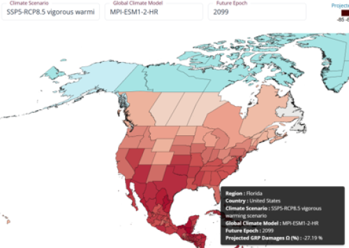
Note: this forecast uses the MPI-ESM1-2-HR model under the SSP5-RCP8.5 vigorous warming scenario. 

Table 2: Florida – EDHEC-CLIRMAP’s projections out to 2099

Cumulative state exposure: Florida leads the US in total cumulative costs (~$450 billion) from billion-dollar disasters since 1980, largely due to hurricanes. Texas is second (~$436 billion) and has been affected by the highest number of billion-dollar disasters. Louisiana’s total is third (~$314 billion).

 

Floods

For inland flooding, a warmer atmosphere holds more moisture, producing more intense rainfall events even in regions not historically prone to flooding. This is what drove West Virginia’s historic 2024 drought-to-flood whiplash, and what makes flash flooding increasingly unpredictable.

For coastal flooding, sea level rise is the primary accelerant. Average sea level has risen over 15cm since 1900 and is expected to rise 30-75cm this century. A study of Hurricane Katrina estimated that higher sea levels led to flood elevations 15–60% higher. A study of Hurricane Sandy estimated that sea levels at the time made severe flooding three times more likely, and that additional rising will make it four times more likely in the future. High tide flooding is now twice as frequent as 20 years ago, and the US is expected to average 45–85 such days per year by mid-century.

• Texas & the Mississippi basin: Inland flooding kills more people each year in the US than storms. Some 1.8 million Texans live in areas with substantial flood exposure. Missouri, Mississippi, and the wider Mississippi River basin suffer from major river overflows due to heavy rainfall and snowmelt.
• Galveston, Texas consistently sees some of the most severe and frequent high-tide coastal flooding of any city in the US. By mid-century, the nation is expected to experience an average of 45 to 85 high-tide flooding days per year. 

 

GRP damage mechanisms 

The mechanisms transmitting flood damage to GDP and GRP include:

Acute Risks

• Direct asset destruction hits property, infrastructure, and cropland simultaneously. Flooding costs the US $179.8 billion–$496 billion annually, equivalent to 1–2% of GDP. Every dollar invested in flood protection saves $5–8 in damages.
• Labour market disruption displaces workers and shuts businesses, with secondary costs from contaminated water and disease.
• Supply chain disruption severs road, rail, and port links, spreading damage nationally. Agricultural supply chain disruption sends price signals through food systems nationally, driving inflation in food sectors even in unaffected regions.
• Sectoral impacts concentrate in real estate, agriculture, and construction, with annual tax revenue losses from flooding estimated at $10.3 billion.

Chronic Risks

• Property devaluation suppresses local tax revenues and reduces household wealth, constraining consumer spending for years.
• Permanent coastal asset erosion, as rising seas expand flood zones, progressively reduces property values and increases event frequency and severity.
• Chronic underinsurance drag: outdated flood maps leave communities systematically underprepared, slowing recovery after each event. Rising premiums and growing uninsurability are beginning to suppress property markets in the most exposed area, with cascading effects on local tax bases and mortgage markets.

Infrastructure degradation, as repeated flooding accelerates wear on roads, bridges, and utilities, requires ever-larger public expenditure with no productive return. Aging US infrastructure needs repairs and added resilience to withstand more frequent and powerful flooding.

A real-world example of the financial impact of chronic flood damage: Hurricane Sandy, 2012  Rising sea levels alone added an estimated $8.1 billion to the damage caused by Hurricane Sandy in 2012, ballooning the flood zone to affect an additional 71,000 people. This is the slow-burn version of flood risk, an accelerating, irreversible loss of coastal asset value driven by rising seas. With no climate adaptation, annual financial damage to US coastal property is forecast to reach $5 trillion through 2100. Research projects that coastal property owners will incur $350 billion in losses between 2060 and 2079, ballooning to $880 billion over the following 20 years

 

Wildfires 

• California, most fires: the 2025 Palisades Fire was one of the most devastating wildfires in the state’s history and destroyed over 6,800 structures.
• Oregon, most acres: More wildfires occur in the East and central states, but western fires are far larger.
• Alaska, high for both: the Arctic is warming 3-4 times faster than the rest of the globe and Alaska has vast tracts of highly flammable black pine forests.

 

Alaska Through the EDHEC-CLIRMAP Lens

Alaska is the fastest warming US state and is seeing surging wildfires as its forest land becomes dryer and warmer. EDHEC-CLIRMAP signals GRP damage of 14% for the state by 2099 (see Figure 2 and Table 3).

Figure 2: Alaska - EDHEC-CLIRMAP shows a 14% GRP impingement by 2099 

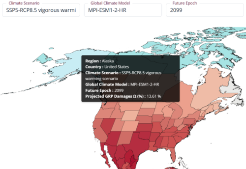
Note: this forecast uses the MPI-ESM1-2-HR model under the SSP5-RCP8.5 vigorous warming scenario. 

 

Table 3: Alaska – EDHEC-CLIRMAP’s projections out to 2099

Note: this forecast uses the MPI-ESM1-2-HR model under the SSP5-RCP8.5 vigorous warming scenario. 

 

Wildfire damage

Wildfire damage falls into three broad categories: economic, health, and environmental. The indirect costs dwarf the direct ones.

Direct structural damage is the most visible. Between 2015 and 2024, wildfires destroyed more than 8,000 structures annually on average. 

Health costs are enormous and geographically dispersed. Wildfires now cause approximately 25% of Americans’ total exposure to harmful fine particulate matter. Wildfire smoke can lead to lost productivity far from the fire’s location and cause premature deaths. 

Economic disruption beyond structures includes: power shut-offs, business closures, travel cancellations, supply chain disruptions, and steep drops in overall employment and surges in unemployment claims in affected regions.

Agricultural and timber losses are substantial: damaged watersheds reduce agricultural productivity, while timber losses represent an economic injury that can take decades, and in some cases up to a century, to reverse.

 

California Through the EDHEC-CLIRMAP Lens

Using the EDHEC-CLIRMAP tool we can see a potential for GRP damage of 27% in California by 2099 (see Figure 3 and Table 4).

Figure 3: California - EDHEC-CLIRMAP shows a 27% GRP impingement by 2099 

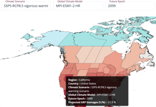
Note: this forecast uses the MPI-ESM1-2-HR model under the SSP5-RCP8.5 vigorous warming scenario. 

 

Table 4: California – EDHEC-CLIRMAP’s projections out to 2099

Note: this forecast uses the MPI-ESM1-2-HR model under the SSP5-RCP8.5 vigorous warming scenario 

 

How climate change is evolving wildfire damage

Warmer, dryer conditions are dramatically extending fire seasons and increasing fire intensity. While the annual number of fire ignitions declined approximately 10% between 1990 and 2024, the annual area burned increased substantially, meaning fewer but far larger and more destructive fires. The insurance system has been hard hit, with some regions now facing uninsurability challenges. Of the nearly $150 billion in damages caused by California’s 2018 wildfires, approximately 60% were indirect economic losses from disruption to economic activity. Under a middle-of-the-road climate scenario, federal fire suppression costs alone are projected to rise 42% by 2050, and that is before accounting for the cascading economic damage that follows each fire.

GRP damage mechanisms 

Wildfires damage regional economies through a set of transmission channels that are unusually broad and deeply interconnected. The immediate destruction of physical capital (homes, businesses, energy infrastructure, and timber) removes productive assets from the economy, while forced evacuations halt economic activity across entire regions even in areas that escape direct burning. The damage then ripples outward: smoke travels thousands of miles, suppressing labour productivity and driving health costs far beyond the fire perimeter. Real estate values fall in affected areas, eroding household wealth, the local tax base, and access to credit simultaneously. Watersheds are contaminated, raising water treatment costs and threatening agricultural productivity for years after the flames are extinguished. Insurance markets come under structural strain as claims surge and insurers withdraw from fire-prone markets entirely, compounding costs for those who remain. 

Acute risks

• Direct asset destruction to property, timber, and infrastructure costs the US $394 billion–$893 billion annually, equivalent to 2–4% of US GDP.
• Labour market disruption is amplified by smoke, which extends far beyond the fire zone. It slashes labour market earnings by an estimated $93 billion per year across the entire US.
• Supply chain disruption dominates the total cost. In California’s 2018 wildfires, indirect supply chain losses accounted for 59% of total damages, dwarfing direct capital losses of 19%.
• Sectoral impacts fall hardest on real estate, insurance, forestry, and tourism.

Chronic risks

• Permanent natural capital erosion as rising fire frequency depresses the long-run value of western forestry, recreation, and watershed services. 
• Persistent air quality drag as smoke seasons lengthen, reducing earnings across manufacturing, healthcare, real estate, and transport.
• Insurance market retreat renders high-risk areas effectively uninsurable, depressing property values and undermining local tax bases over the long term.

A real-world example of the financial impact of acute wildfire damage: Los Angeles Fires, January 2025 Driven by exceptional Santa Ana winds and prolonged drought conditions, the Palisades and Eaton fires tore through Los Angeles County in January 2025, destroying more than 16,000 structures. Insured losses alone amounted to $40 billion, making them the costliest wildfires on record globally, and total economic loss to $250 billion–$275 billion. Property and capital losses of $76 billion–$131 billion helped fuel a 0.48% decline in county-level GDP for 2025, equivalent to approximately $4.6 billion.

 

Droughts and heatwaves

Historically, drought in the Western US states has been caused by lack of precipitation, with evaporative demand playing a smaller role. Rising temperatures have shifted this balance: droughts induced by natural fluctuations in rainfall continue, but there is more heat to suck moisture from bodies of water, plants, and soil.

Alaska and the desert Southwest are the fastest-warming and most chronically drought-stricken states. But 2024 revealed a new and alarming pattern; states like West Virginia, Ohio, and across the Northeast – that have never historically faced serious drought – are now seeing record conditions. Climate change is no longer just a Western story.

The chronic drought states are the usual suspects in the Southwest. Far West Texas, southern New Mexico, and the Northern Rockies remained in persistent drought throughout all of 2024. 

Nevada is the number one state for drought risk in the Southwest, facing increased heat waves and water evaporation, with the Colorado River, which supplies water to millions, under severe threat from reduced flow.

But the alarming 2024 story is in the East, where drought struck with shocking speed. West Virginia experienced its worst drought in at least two decades. During one week in June, drought coverage increased ten-fold, and by mid-August 99% of the state was in drought. Ohio and West Virginia saw their greatest area in Extreme and Exceptional Drought since the US Drought Monitor began in 2000.

 

Texas Through the EDHEC-CLIRMAP Lens

EDHEC-CLIRMAP shows alarming GRP damage of 43% for the state of Texas by 2099 (see Figure 4 and Table 5).

Figure 4: Texas - EDHEC-CLIRMAP shows a 43% GRP impingement by 2099

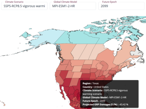
Note: this forecast uses the MPI-ESM1-2-HR model under the SSP5-RCP8.5 vigorous warming scenario 

 

Table 5: Texas – EDHEC-CLIRMAP’s projections out to 2099

Note: this forecast uses the MPI-ESM1-2-HR model under the SSP5-RCP8.5 vigorous warming scenario 

The wet-bulb temperature threshold: too hot for humankind “Wet-bulb temperature” is a measure that combines heat and humidity, reflecting how effectively a person can cool themselves by sweating. Some coastal subtropical areas have already experienced conditions at or near humans’ survivability limit at 35°C.  The southeastern US, especially along the Gulf of Mexico, has had multiple incidences of wet-bulb temperatures at or above 31°C, specifically in east Texas, Louisiana, Mississippi, Alabama, the Florida Panhandle, Arkansas, and North Carolina. Serious health impacts occur at wet-bulb temperatures as low as 26°C.  In October 2024 abnormal dryness and drought affected over 78% of the American population, the highest percentage in the Drought Monitor’s 25-year record. As of 1 September 2026, 49.51% of the United States and Puerto Rico and 59.05% of the Lower 48 states were in drought. One striking pattern: in most of the US, including all Northeastern, Southeastern, and Midwestern states, winter is the fastest-warming season. In Vermont, winters alone have warmed by around 4.5°C since 1970.

Table 6: The fastest-warming states 

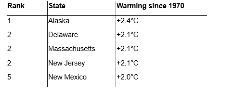
Source: Climate Central’s Earth Day Warming Rankings (1970–2024) , which draws on NOAA/NCEI Climate at a Glance .

 

GRP damage mechanisms 

Droughts are the second-costliest natural disaster in the US after hurricanes. The agricultural sector is historically the most sensitive; drier soils and reduced water availability damage yields, leading to lost farm income, seasonal labour displacement, and supply chain disruptions. A 2019 study found that an additional week of drought could cause up to an 8% reduction in corn yields. For livestock, dry pastures mean expensive supplemental feed and transporting water for animals. 

The 1988–1989 drought led to crop losses valued at $15 billion. California’s 2014–2016 drought caused $2 billion in crop losses, $553 million dairy and livestock losses, and $1.3 billion in additional groundwater pumping costs in those three years alone.

Acute risks

• Labour productivity decline is the primary transmission mechanism for heatwaves. Extreme heat and severe droughts reduce GDP by around 0.2%, larger than many economists previously calculated. Heat-related productivity losses grew from a model average of $130 billion in 2001 to $220 billion in 2023, a 70% increase in just two decades. The trajectory is alarming: without emissions reductions or sufficient heat adaptations, labour productivity losses may double to nearly $200 billion by 2030 and reach $500 billion by 2050.
• Direct output loss across agriculture, energy, and water-intensive industry produce GDP losses of around −2% over four years, the most persistent negative GDP effect of any weather disaster type
• Supply chain disruption is amplified when drought and heat coincide, with Mississippi river transport disruptions alone estimated at $20 billion in losses.
• Sectoral impacts concentrate in agriculture and energy, with GDP effects persisting for up to six quarters, longer than any other acute weather event.

Chronic risks

• Structural labour productivity erosion as rising baseline temperatures permanently reduce outdoor working hours, with some Texas and Florida counties projected to lose over 6% of labour hours annually by 2100.
• Agricultural output decline compounds over time, with each 1°C of warming associated with a 5–15% decrease in crop production and potential 25% losses in Midwest output by 2050.
• Compounding fiscal pressure from recurring relief spending and water infrastructure investment crowds out productive public expenditure. Prolonged drought drives inflationary pressures, recessions, slower long-term GDP growth, and rising fiscal deficits.

As with hurricanes: acute damage can be partially offset by reconstruction spending, while chronic damage accumulates without an equivalent rebound.

 

A real-world example of the financial impact of chronic heat & drought:  The Western Megadrought, 2000–present The American West has been locked in its driest 22-year period for at least 1,200 years, fuelled by human-caused warming. The financial toll is cumulative and structural: from 2011-2020 alone, the US experienced nine droughts each causing at least $1 billion in damages. The 2012 peak, the worst drought year since the 1930s, cost over $30 billion. The USDA declared a natural disaster across 2,245 counties, covering 71% of the US. Looking forward, the poorest third of US counties are projected to experience climate damages costing 2-20% of county income under a high emissions scenario.

Conclusion: discussing the true damage figure does not negate the threat

As our climate is changing, tools that translate physical risk into economic impacts are becoming increasingly important. Combining macroeconomic modelling, climate econometrics and the Delta method, EDHEC-CLIRMAP allows users to explore the spatial distribution of projected economic damages and their heterogeneity, supporting investment analysis and adaptation planning.

These estimates should nevertheless be interpreted as partial measures of risk. Current damage functions and integrated assessment models often do not fully capture cascading failures, threshold effects, compound shocks or climate tipping points. In particular, many models assume that damages increase smoothly with temperature, while some physical and economic impacts may become non-linear beyond certain warming levels.

This limitation is especially relevant for compound events. A wildfire following a drought and heatwave, or a storm affecting a coastal city already exposed to sea-level rise, can generate larger and more persistent losses than the same hazard considered in isolation. Future research therefore needs to better account for interacting hazards, tipping points and propagation channels across regions and sectors.

The implication is that the damage estimates discussed in this article, while already material, may remain conservative.

 

The next step: Addressing a structural blind spot in sovereign pricing with the Sovereign Climate Risk Rating (SovCRR)

EDHEC-CLIRMAP is a genuinely flexible resource for investors and researchers seeking to gauge the relationship between a warmer climate and economic output. It’s supported by 50 years of granular data across more than 1,600 regions, incorporates NASA climate models across 3,672 global regions worldwide. It can help resolve forward-looking questions about climate-driven economic change, making it reusable well beyond its own map interface.

Sovereign climate-risk measures, for instance, tend to typically begin with country averages and end in composite scores. The Sovereign Climate Risk Rating (SovCRR) follows the opposite route. It begins with the econometric architecture or scientific bedrock underlying EDHEC-CLIRMAP and thus uses historical temperature and output records observed at the sub-national level prior to project the resulting damages across more than 3,400 regions. SovCRR then translates those estimates into nine probabilistic pathways aligned with the NGFS, and only then aggregates them into a probability-weighted country-level expected loss or gain that feeds into an A–G rating. The letter grade is an important reporting layer; beneath it lies a transparent, scenario-consistent and probability-weighted estimate of the future impact of chronic physical climate risk on GDP per capita. 

The result is what makes these ratings valuable to investors: a forward-looking, probability-weighted, economically interpretable number, built from the ground up rather than a single national average. That sub-national foundation matters in practice, because, as we have explored in this note, a country’s climate exposure is very rarely uniform: aggregating from the region up, the way CLIRMAP does, catches concentrated risk in an economy’s hottest, most populous areas that a country-level model would dilute away.