How can we quantify the potential equity portfolio losses that may be attributed to physical climate risk in the future? Over recent years, it has become increasingly important for pension funds and other investors to answer this question in ways that are credible, transparent, and in tune with regulators’ requirements. In this article (a summary of a recent paper[1]), we examine the U.S. equity market using a ‘Climate Physical Loss (CPL)’ framework. The methodology is top-down, parsimonious, based on public data, and aligned with the NGFS scenario set[2]. Importantly, it is also directly applicable to asset allocation and portfolio construction due to its use of a discounted-cash-flow model and, therefore, of practical use to investors seeking not simply an assessment framework but a useable portfolio management tool.
This article explicitly focuses on U.S. equities, while the accompanying article (Quantifying Climate Physical Loss and Heterogeneity: European Equities) investigates the case of European equities.
Key takeaways
- We find that U.S. states on average exhibit higher macroeconomic sensitivity to physical climate risks than Developed Europe, although there is a huge amount of heterogeneity between sectors and between states, with larger projected deviations of nominal GDP in southern regions (e.g., -48.6% in Florida by 2100 under the NGFS ‘current policy’ scenario).
- However, the U.S. cap-weighted equity benchmark displays a smaller Climate Physical Loss (CPL) of -4.0%, versus-4.7% for Europe.
- This apparent dampening effect is primarily driven by benchmark composition, with the U.S. equity market more exposed to high-WACC, lower-sensitivity sectors and less concentrated in physically vulnerable regions than its European counterpart. As such, the research highlights the importance of portfolio construction in determining resilience.
Introduction: quantifying physical climate risk
Physical acute climate hazards such as heatwaves, floods, droughts, storms and or chronic sea-level rise increasingly represent a challenge for firms and governments, as well as financially material risks for investors. Regulatory and supervisory authorities increasingly acknowledge that physical climate risks must be systematically integrated into risk management frameworks. The recommendations of the Task Force on Climate-related Financial Disclosures (TCFD), followed by the issuance of the International Sustainability Standards Board’s IFRS S2 standard, have formalized the requirement to identify and disclose material physical and transition risks, underpinned by robust scenario analysis.
In the United States, the regulatory treatment of climate-related financial risk remains more fragmented and contested than in the European Union, but supervisory authorities have nevertheless acknowledged that the risks may already be financially material and warrant forward-looking assessment. In March 2024, the Securities and Exchange Commission (SEC) adopted a climate-related disclosure rule requiring large public companies to disclose material climate risks and their financial impacts (SEC, 2024), though the rule has been stayed following legal challenges, leaving its implementation uncertain.[3]
In parallel with regulatory developments, an extensive academic literature has emerged to demonstrate how climate-related risks are reflected in asset prices and establish forward-looking methodologies such as short-term stress tests and long-term scenario analyses (which typically rely on integrated assessment models to quantify climate-related value-at-risk or evaluate changes in discounted cash flows under alternative temperature or policy pathways). However, these analyses are generally conducted at high levels of geographic and macroeconomic aggregation. While these are well suited for large systemic risk assessments, investors lack further information granularity for strategic investment management. This is particularly true when it comes to U.S. states whose differential exposure to physical risk—although intuitive—is systematically averaged out by climate scenario providers (in search of national and global metrics).
As such, this article presents a methodology that is directly applicable to institutional investors and asset managers who are looking to understand CPL for their own equity portfolios. This approach has the advantage of providing intra-U.S. answers through a transparent and intuitive framework, without imposing onerous or resource-intensive data requirements.
Building and calibrating a ‘CPL’ framework
The proposed Climate Physical Loss (CPL) framework rests on the principle that physical climate risk affects firm value through its impact on macroeconomic activity and, ultimately, on expected future cash flows. As such, a firm-level CPL is the difference between a firm’s baseline enterprise value and an alternative valuation in which future cash flows are scaled by macroeconomic losses attributable to physical climate risks.
Formally, the procedure consists of three steps: (i) quantifying regional (country- and U.S. state-level) GDP losses as a function of temperature anomalies; (ii) transmitting these losses to firm valuations through a discounted‑cash‑flow framework; and (iii) reweighting relative valuation losses using sector‑level sensitivity scores.
Step 1: estimating regional GDP losses as a function of temperature anomalies
Country- and U.S. state-level macroeconomic projections are sourced to obtain both the baseline trajectory of aggregate economic activity and the deviations from this trajectory induced by temperature anomalies. Country-level deviations are based on the NGFS scenario set[4], while state-level disaggregation (relating to each state’s economic weight and exposure to physical climate risks) uses sub-national damage projection outputs from the EDHEC Climate-Induced Regional Macro-Impacts Projector (EDHEC-CLIRMAP) database.
The global non-linear effect of temperature on economic production has been empirically confirmed by Burke et al. (2015) and Newell et al. (2021), providing evidence for an inverted U-shaped relationship whereby temperatures exceeding a turning point generate amplifying reductions in per capita GDP. We first estimate a damage function at the most aggregated-level for the U.S. (i.e., national), linking physical risk-induced U.S.-level GDP damages (arising from both chronic and acute climate risk) to a non-linear function of global temperature anomalies, as emulated by NGFS MAGICC across scenarios and IAMs,

where global temperature anomaly  is measured relative to a reference year
  and where
  denotes the percentage deviation of real GDP from a no-damage baseline.
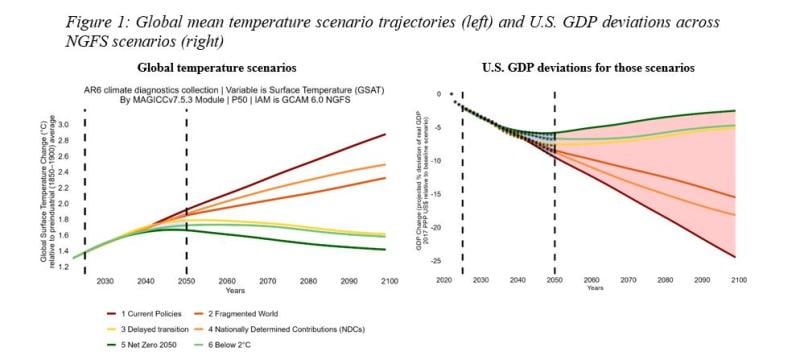
Figure 1: Global mean temperature scenario trajectories (left) and U.S. GDP deviations across NGFS scenarios (right)
Data from NGFS, IPCC. Interpolation under GCAM 6.0 NGFS IAM. LHS: Global surface temperature (GSAT) projection from the MAGICCv7.5.3 climate model, based on AR6 climate diagnostics used by NGFS Phase-V. RHS: NiGEM-projected annual GDP changes from physical impacts for 2022–2050 are represented by the stars. The GDP deviations obtained in this study, shown as continuous splines, ultimately coincide with those from NiGEM over the matching time frame, prior to extrapolation through 2100. For robustness check, GDP deviations are normalized to 2022 instead of the usual 2025 reference year.
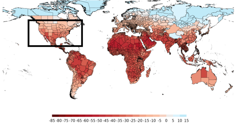
Figure 2: Spatially distributed region-level projected damages (%) to per capita GDP, 2099
Data from EDHEC-CLIRMAP. Estimates from multi-model medians of 15 ’likely’ CMIP6 GCMs, epoch 2099 relative to historical 1985-2004 temperature means, according to a synthetic intermediate mid-point scenario between SSP5-8.5 vigorous & SSP2-4.5 moderate warmings. Projected damages across time (20-year centered moving averages, 2030–2099) and geographies underpin the climate loss factor used in this article. Source: Schneider (2025).
Because NGFS only provides estimates of GDP deviations relative to a baseline scenario at the country level, we introduce state-level heterogeneity through state-specific climate loss factors, thereby disaggregating national damages to the sub-national level. These climate loss factors correspond to the relative economic damage per U.S. state related to the current state (not to a baseline scenario), as provided by an external database of macroeconomic damages: EDHEC-CLIRMAP[5]. This procedure is done to ensure maximum consistency between the NGFS U.S. country damages and the regional damage.
Let be  the climate loss factor per state, and a time-varying calibration parameter
  ,
,

The calibration factor , is computed to ensure that the GDP-weighted sum of state damages equals the national damage estimated earlier:

Where  represents state
  ' share of total U.S. GDP (20-year centered moving average). This approach ensures perfect aggregation (
 ) while allowing state damages to scale proportionally with their climate vulnerability factors. The calibration parameter varies over time, enabling the relative magnitude of state-level impacts to evolve with the US-level climate response.
From the estimated aggregate damage function, nominal GDP growth factors under the baseline and physical-risk scenarios are defined as

where  denotes the aggregate price level. These factors scale firm-level cash flows in the valuation stage.
Step 2: Transmitting these losses to company valuations through a DCF model
The next stage is to incorporate those deviations into a discounted-cash-flow (DCF) model: firm-level cash flows are assumed to grow with state nominal GDP and are discounted using sector-specific weighted average costs of capital (WACC).
The discount rates used in the discounted cash flow model are obtained from Damodaran’s publicly available estimates, which provide industry-level values for different regions[6].
From a model construction perspective, we can let firms be indexed by  , and denote by
  the state of firm and by
  its sector. Cash flows in the reference year are given by
  . For horizon
  to
to  , the baseline enterprise value follows[7]

where  is the sector- and region-specific discount rate (weighted average cost of capital). Under the physical-risk scenario:

Since is common to both valuations, the relative enterprise value loss simplifies to

Thus,  , our primary impact metric, measures the proportional decline in firm value solely attributable to physical risk-induced damages.
Step 3: Reweighting relative valuation losses using sector‑level sensitivity scores
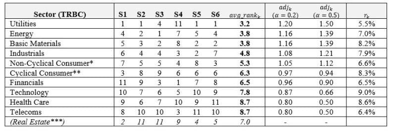
In the third stage, a final adjustment is applied to reflect the prevailing market assessment of the sensitivity of different sectors to physical climate risk. Various ESG data providers report scores measuring sectors’ perceived vulnerability to physical climate risk. Our model incorporates empirical evidence from Hain, Kölbel, and Leippold (2022), who compare six firm-level physical risk scores from commercial and academic sources. Although the providers differ markedly in methodology, the authors document substantial systematic variation across sectors: Utilities, Energy, and Materials consistently appear as the most exposed sectors, while Health Care, Communication Services, and Information Technology exhibit comparatively low exposure. This data is used to produce a sector-adjusted relative enterprise value loss, such that losses are scaled upward in highly exposed sectors and downward in less exposed sectors[8].
Figure 3: Sector-specific characteristics
The seven first columns of this table from Hain, Kölbel, and Leippold (2022). They show sector rankings of six different ESG data providers based on the sensitivity of sectors to climate physical risks: Trucost (S1), Carbon4 Finance (S2), Southpole (S3), Truvalue Labs (S4), Sautner et al. (S5), and Kölbel et al. (S6).
Results: how exposed is the U.S. market to physical climate risks?
Using the above model, we conducted empirical analysis focused on the 500 largest publicly listed U.S. firms. This allowed us to assess:
- The heterogeneous climate physical risk sensitivity of U.S. states;
- how sector-specific discount rates and sector-level exposure to physical hazards affect outcomes; and
- implications for U.S. equity portfolio valuation.
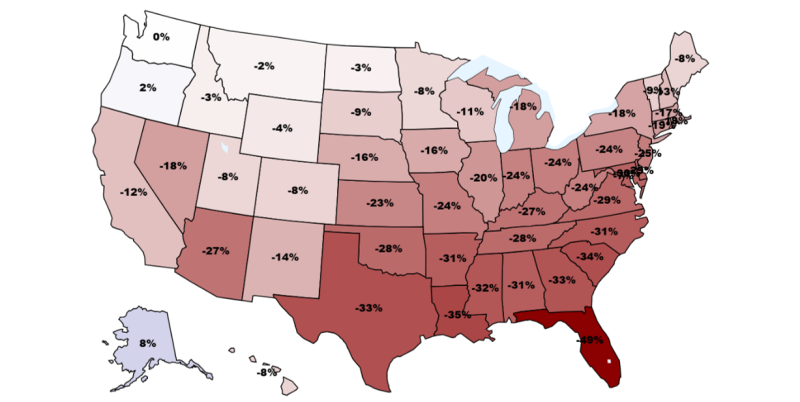
Across the 50 U.S. states, projected long-term economic outcomes exhibit substantial heterogeneity, ranging from an estimated gain of around 8% for Alaska to a loss of approximately 49% for Florida. These differences are strongly correlated with latitude: southern states face markedly larger economic losses, a pattern in good agreement with the general literature on this topic (Burke et al., 2015; Kalkuhl and Wenz, 2020; Linsenmeier, 2023; Kotz et al., 2024; Schneider, 2025; Bilal and Känzig, 2026).
Figure 4: Projected nominal GDP loss by 2100 under current policies for U.S. states
The figure reports, for each U.S. state, the projected relative loss in nominal GDP in 2100 under the NGFS Current Policies scenario (GCAM model), expressed as a percentage deviation from the corresponding baseline trajectory.
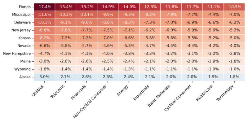
Next, we look at sector-level heterogeneity. Sectors such as Utilities or Non-Cyclical Consumer—which typically exhibit relatively low WACC—are valued on the basis of long-term cash-flows and are therefore more exposed when the distant flows are impacted by physical risks. Conversely, high-WACC sectors such as Technology are priced primarily on near-term cash flows, which makes their valuations less sensitive to physical risk shocks affecting distant cash flows. Incorporating this sectoral adjustment generates substantial dispersion in climate-induced valuation effects, with a ratio of approximately 1.6 between the most and least sensitive sectors (Figure 5).
Figure 5: Effect of sector-specific discount rate only on climate physical loss (CPL)
The heatmap displays the climate physical loss (CPL) for a selection of 10 U.S. state–sector pairs after incorporating sector-specific discount rates. Sectors with low weighted average cost of capital tend to exhibit higher CPL as they are more sensitive to the long-term impact of climate change on their cash flows. Results are based on the NGFS “Current Policies” scenario, using the GCAM model at the 2100 horizon.
A second sectoral adjustment concerns the sectors’ perceived vulnerability to physical climate risks: certain sectors are more vulnerable to physical risks (e.g., Utilities, Energy, and Materials[9]). Because the initial degree of vulnerability is specified in terms of a ranking, its conversion into a valuation relies on an additional parameter α that can take different values to modulate the influence on the final CPL. As  is difficult to estimate empirically, the analysis evaluates the sensitivity of results to alternative values, focusing on
  and
and  as plausible bounds. Results show that varying α not only alters the magnitude of CPL within a given state but may also change the ordering of the most affected sectors. This arises from the interaction with the discount-rate effect. For some sectors, such as Utilities, a relatively low discount rate is compounded by high vulnerability (i.e., a high adjustment factor) identified in the literature, whereas for other sectors, such as Financials, the effect of a low discount rate is dampened by their relatively low perceived vulnerability to physical risks[10].
Application to a U.S. equity benchmark
Within the sample of U.S. states and sectors, the estimated climate physical loss (CPL) spans a wide range, from –26.2% to +4.5% ( ). Portfolio-level exposure is therefore highly sensitive to the underlying region and sector allocation. For the U.S. cap-weighted equity benchmark, the weighted CPL amounts to –4.0%.Exhibit 6illustrates how alternative state- and sector-weightings would influence this result. It is evident that the benchmark’s sector allocation highly mitigates physical risk exposure, and that this effect is amplified by the state-allocation effect. This latter can be traced back to the overweight positions in U.S. states with lower physical-risk exposure.
Exhibit 6: Climate physical loss of the U.S. equity benchmark
The table reports the weighted climate physical loss (CPL) under alternative allocations. “Equal” allocates identical weights to each of the 50 U.S. states (or 10 sectors) in the sample, while “Portfolio” applies the weights of the U.S. equity benchmark to the corresponding states or sectors.
This framework offers a basis for producing estimates of ‘Climate Physical Loss (CPL)’ for U.S. equities through a parsimonious, transparent and NGFS-aligned approach, but is not without caveat.
We empirically show that estimated sensitivity parameters that structure the U.S. aggregate damage function in Step 1 are robust to the choice of NGFS scenario or integrated assessment model (IAM) and thus, scenario- and IAM-invariant[11]. This reflects the fact that IAMs operating under a given scenario must satisfy broadly similar aggregate carbon-budget constraints over the period. By contrast, while scenario selection is only modestly influential over outcomes over short time horizons (see the relatively narrow inter-scenario range depicted by the blue-shaded area circa-2050 in Figure 1), it becomes highly influential over long time horizons (as one would perhaps expect from Figure 1) since scenario-trajectories substantially diverge.
Conclusion: from climate risk assessment to strategic investment decision making
Investors are increasingly required to provide robust assessments of the potential impact of physical climate risks on their equity portfolios. We contend that (1) it is feasible to perform these assessments in a parsimonious and regulator-compliant manner, without the need for asset-level or physical hazard data that creates an excessive burden on resources; and (2) that these assessments can be done in an operationalized manner, making them directly transferable to strategic investment decision-making. We believe that the framework presented here achieves both (1) and (2) simultaneously. Moreover, the findings generated from this framework strongly showcase the importance of portfolio construction (i.e., accounting for the heterogeneous exposure of sectors and economic regions distributed intra-country) in altering resilience to global temperature trajectories.
Footnotes
[1] Physical Climate Risk in the U.S. Equity Market: Quantifying State-Sector Heterogeneity, Bouchet, V., Schneider, N. (2026b)
[2] NGFS Scenarios Portal, Network for Greening the Financial System
[3] Reuters. 2025. “U.S. SEC Votes to Stop Defending Climate Disclosure Rules.” March 27, 2025.
[4] The U.S. economic sensitivity to a non-linear function of global temperature anomalies,  and
and  is estimated using the NGFS Phase 5 scenario dataset. This provides combinations of qualitative transition narratives and quantitative outputs from integrated assessment models (IAMs) that generate transition and physical-risk dynamics (e.g., REMIND, MESSAGE). For each scenario–model configuration, the NGFS reports projected country-level paths of real GDP. Rather than using these GDP projections directly, the dataset is used to re-quantify the relationship between global temperature anomalies and deviations of country-level GDP from baseline. Long-horizon nominal GDP projections are derived from two components: (i) a baseline scenario that represents the path of economic activity in the absence of climate damages through 2100, and (ii) a physical-risk scenario in which global temperature anomalies are mapped into country-level economic losses. For long-term projections (post-2050), the baseline real-activity path combines projections from the NGFS and the IPCC–SSP2 framework. Country-level deviations are generated by applying the estimated damage coefficients to an exogenous global mean temperature (GMT) trajectory. The sequence of global temperature anomalies is inserted into the quadratic damage function above to obtain non-linear and country-specific GDP deviations
  . When combined with the baseline GDP trajectory, these deviations yield the physical-risk and baseline GDP growth factors,
  and
and  , which in turn determine the evolution of firms’ expected cash flows. For more information, see Physical Climate Risk in the United States Equity Market: Quantifying State-Sector Heterogeneity (Bouchet & Schneider, 2026a)
[5] This is a proprietary EDHEC research building on Schneider (2025). Details on the quantitative methodology underlying this module are provided in §2.2 Data and model calibration.
[6] Firm-specific discount rates are computed by assigning each TRBC sector to the appropriate set of Damodaran industry classifications. Information on the sector and country classification of stocks is sourced from CIQ, while the portfolio weights of stocks are taken from the Scientific Portfolio Capital Weight Regional Benchmark for United States.
[7]  is assumed to be far enough in the future to make any terminal value relatively negligible after discounting.
[8] Again, for more details on the integration of these sensitivity scores into the enterprise value loss calculation, see Physical Climate Risk in the United States Equity Market: Quantifying State-Sector Heterogeneity (Bouchet & Schneider, 2026a)
[9] Data are taken from Hain, Kölbel, and Leippold (2022).
[10] For tables showing the results for this analysis, see Physical Climate Risk in the United States Equity Market: Quantifying State-Sector Heterogeneity (Bouchet & Schneider, 2026a)
[11] See Physical Climate Risk in the United States Equity Market: Quantifying State-Sector Heterogeneity (Bouchet & Schneider, 2026a). Complementary results from this robustness test, performed on Eurozone data, may also be found in: Physical Climate Risk in the European Equity Market: Quantifying Country-Sector Heterogeneity (Bouchet & Schneider, 2026b)
References
- Bilal, A., & Känzig, D. R. (2026). The Macroeconomic Impact of Climate Change: Global Versus Local Temperature. The Quarterly Journal of Economics, qjag011.
- Bouchet, V., & Schneider, N. (2026a). Physical Climate Risk in the United States Equity Market: Quantifying State – Sector Heterogeneity. Scientific Portfolio-an EDHEC Venture White Paper.
- Bouchet, V., & Schneider, N. (2026b). Physical Climate Risk in the European Equity Market: Quantifying Country – Sector Heterogeneity. Scientific Portfolio-an EDHEC Venture White Paper.
- Burke, M., Hsiang, S. M., & Miguel, E. (2015). Global non‑linear effect of temperature on economic production. Nature, 527(7577), 235–239.
- Kalkuhl, M., & Wenz, L. (2020). The impact of climate conditions on economic production: Evidence from a global panel of regions. Journal of Environmental Economics and Management, 103, 102360.
- Kotz, M., Levermann, A., & Wenz, L. (2024). RETRACTED ARTICLE: The economic commitment of climate change. Nature, 628(8008), 551-557.
- Linsenmeier, M. (2023). Temperature variability and long-run economic development. Journal of Environmental Economics and Management, 121, 102840.
- Schneider, N. (2025). The Global Geography of Long-Term Projected Macroeconomic Damages from Chronic Physical Risk and the Aggregation Problem. SSRN Working Paper. Available at https://ssrn.com/abstract=5630697.